Probabilistic Spiking Neuronal Nets: Companion
Table of Contents
- 1. Introduction
- 2. Chapter 2 Material
- 3. Appendix A Material
- 3.1. The inter mepp data of Fatt and Katz (1952)
- 3.2. Exercise 1: Getting the data
- 3.3. Exercise 2: Basic statistics
- 3.4. Exercise 3: Interval correlations
- 3.5. Exercise 4: Counting Process Class
- 3.6. Exercise 5: Graphical test of arrival times 'uniformity'
- 3.7. Exercise 6: Kolmogorov's test via
Ccode interfacing (optional) - 3.8. Exercise 7: Figure 12 reproduction and more
- 3.9. Solution 1: Getting the data
- 3.10. Solution 2: Basic statistics
- 3.11. Solution 3: Interval correlations
- 3.12. Solution 4: Counting Process Class
- 3.13. Solution 5: Graphical test of arrival times 'uniformity'
- 3.14. Solution 6: Kolmogorov's test via
Ccode interfacing - 3.15. Solution 7: Figure 12 reproduction and more
1. Introduction
This site contains material associated with the book: Probabilistic Spiking Neuronal Nets – Data, Models and Theorems by Antonio Galves, Eva Löcherbach and Christophe Pouzat (Springer, 2024).
1.1. Type of exercises
You will find here numerical exercises coming in different "flavors" to which tags are associated:
- coding exercises
- require a minimal programming experience and consist in developing some code (writing a function, a program, a script).
- simulation exercises
- consist in running a simulation code (usually developed in a coding exercise) and perform some basic analysis on the result; this requires only basic computer skills like calling a program.
- projects
- something more extensive (taking obviously more time) leading for instance to the reproduction of the simulations and figures of one of the book chapter.
Solutions are systematically provided in Python (supplemented by NumPy and matplotlib). Solutions in a compiled language like Fortran or C will also be provided for comparison, speed and stability in time (Python is great but evolves much too fast giving rise to severe stability issues).
A minimal familiarity with Python is assumed, at least at the level of the official tutorial (a great and fun read!); reading the first chapters of Goodrich, Tamassia and Goldwasser, Data Structures and Algorithm in Python (2013), is highly recommended.
1.2. Figures
The codes generating (most of) the book figures are provided.
1.3. Code presentation
Since the codes can be a bit long from time to time, the literate programming approach will be used. This means a program or script will often be broken into "manageable" pieces, called code blocks, that are individually explained (when just reading the block is not enough). These code blocks are then pasted together to give the program/script. These manageable pieces are given a name like: <<name-of-the-block>> upon definition. Each piece is then referred to by this name when used in subsequent code blocks. See Schulte, Davison, Dye and Dominik (2012) A Multi-Language Computing Environment for Literate Programming and Reproducible Research for further explanations.
Many examples and solutions assume that you have a copy of the code directory (and of its content) in your Python working directory (what is returned by os.getcwd).
1.4. Acknowledgments
Antonio Galves was partially supported by the Brazilian National Council for Scientific and Technological Development (CNPq ) grant number 314836/2021-7. Eva Löcherbach and Christophe Pouzat have been supported by the French National Research Agency (ANR-19-CE40-0024, ANR-22-CE45-0027-01) through the ChaMaNe (E.L.) and SIMBADNESTICOST (C.P.) projects.
2. Chapter 2 Material
2.1. A versatile discrete simulator (project)
Write a versatile simulator covering the different models of Chap. 2 and more. See the dedicated page to read either as a detailed description of a code or as a set of small exercises leading to the code development. (In progress)
2.2. A cross-correlation histogram function (coding exercise)
Write a Python function returning the cross-correlation histogram (or cross-correlogram) associated with two observed spike trains. We use the definition of Brillinger, Bryant and Segundo (1976) Eq. 13, p. 218 (see also Perkel, Gerstein and Moore (1967)). These cross-correlation histograms are estimators of what Cox and Lewis (1966) call a cross intensity function. More precisely, given:
- a simulation/observation window \([0,t_{obs}]\), chosen by the experimentalist,
- the spike trains of two neurons, \(i\) and \(j\): \(\{T^i_1,\ldots,T^i_{N^i}\}\) and \(\{T^j_1,\ldots,T^j_{N^j}\}\), where \(N^i\) and \(N^j\) are the number of spikes of neurons \(i\) and \(j\) during the observation time window (notice that the two neurons are identical, \(i=j\), when we are dealing with an auto-correlation histogram),
- a maximum lag, \(0 < \mathcal{L} < t_{obs}\) (in practice \(\mathcal{L}\) must be much smaller than \(t_{obs}\) in order to have enough events, see below),
- \(K^i_{min} = \inf \left\{k \in \{1,\ldots, N^i\}: T^i_k \ge \mathcal{L}\right\}\),
- \(K^i_{max} = \sup \left\{k \in \{1,\ldots, N^i\}: T^i_k \le t_{obs}- \mathcal{L}\right\}\),
- an integer \(m \in \{m_{min} = -\mathcal{L}, \ldots, m_{max} = \mathcal{L}\}\),
the correlation histogram between \(i\) and \(j\) at \(m\) is defined by: \[ \widehat{cc}_{i \to j}(m) \equiv \frac{1}{\left(K^i_{max} -K^i_{min}+1\right)} \sum_{k = K^i_{min}}^{K^i_{max}} \sum_{l=1}^{N^j} \mathbb{1}_{\{T^j_l - T^i_k = m\}} \, . \]
We have by definition the following relation: \[\left(K^i_{max} -K^i_{min}+1\right) \widehat{cc}_{i \to j}(m) = \left(K^j_{max} -K^j_{min}+1\right) \widehat{cc}_{j \to i}(-m)\, .\] When we are dealing with auto-correlation histograms (\(i=j\)), we have therefore: \[\widehat{cc}_{i \to i}(m) = \widehat{cc}_{i \to i}(-m)\, .\] By construction: \(\widehat{cc}_{i \to i}(0) = 1\) The term "correlation" is a misnomer here, since the means are not subtracted (therefore the estimated quantities cannot be negative): following Glaser and Ruchkin (1976), Sec. 7.2 the term "covariance" would have been more appropriate. You can therefore write a function that computes the correlation histogram only for lags that are null or positive.
Your function should take the following parameters:
- a list or array of strictly increasing integers containing the discrete spike times of the "reference" neuron (neuron \(i\) above).
- a list or array of strictly increasing integers containing the discrete spike times of the "test" neuron (neuron \(j\) above).
- a positive integer specifying the maximum lag.
Your function should return a list or array with the \(\widehat{cc}_{i \to j}(m)\) for m going from 0 to the maximum lag.
You should apply basic tests to your code like:
- Generate a perfectly periodic spike train, say with period 5, compute the auto-correlation histogram: \(\widehat{cc}_{i \to i}(m)\) and check that would get what is expected (you must figure out what is expected first). Notice that a "perfectly periodic spike train" can be modeled with a slight extension of the framework presented in Sec. 2.3, Introducing leakage. We must allow for a self-interaction and take for \(g_i(t-s)\) (Eq. 2.7): \(\mathbb{1}_{t-s=5}\) combined with an identity rate function: \(\phi_i(x) = x\).
- Generate a periodic spike train, say with period 5, that exhibits a spike (at the prescribed times) with a probability say 0.5, compute the auto-correlation histogram: \(\widehat{cc}_{i \to i}(m)\) and check that would get what is expected (you must figure out what is expected first). In line with the previous test, we can fit such a non-deterministic periodic train within the "extended" framework of Chap. 2 by taking: \(g_i(t-s) \equiv 0.5 \, \mathbb{1}_{t-s=5}\).
- Generate two "geometric" (that is with inter spike intervals following a geometric distribution) and independent at first trains,
refandtest, that have a probability 0.05 to exhibit a spike at any given time. For every spike inrefadd a spike in test (if there is not already one) 3 time steps later with a probability 0.5. Compute \(\widehat{cc}_{\text{ref} \to \text{test}}(m)\) and \(\widehat{cc}_{\text{test} \to \text{ref}}(m)\) and check that you get what is expected (you must figure out what is expected first). In the framework of Chap. 2, the presynaptic neuron has a constant rate function \(\phi_{pre}(v) = 0.05\), while the postsynaptic neuron has a \(\phi_{post}(\,)\) function satisfying \(\phi_{post}(0) = 0.05\) and \(\phi_{post}(1) = 0.5\), combined with a \(g_{post}(t-s) \equiv \mathbb{1}_{t-s=3}\).
Once you are done, go to the solution page.
2.3. Exploring a classic 1 (coding exercise)
We will now start a set of exercises based on an article by Moore, Segundo, Perkel and Levitan (1970) Statistical Signs of Synaptic Interaction in Neurons. We first do the simulation leading to Fig. 1 of the paper. Your task is to simulate two neurons, A and B to stick to the labels used by Moore et al, where A is presynaptic to B (a bit like our last test in the previous exercise).
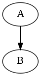
Neuron A discharge is "periodic"—in the sense that it tends to produce regular inter spike intervals—; neurophysiologist call such neurons pacemaker neurons, they can be easily found in invertebrate ganglia like the visceral ganglion of Aplysia californica from which the actual recording of Moore et al paper were made. One way to produce such a discharge is to simulate a process whose spike probability at time \(t\) depends on the elapsed time since the last spike (the \(L_t\) of Eq. 2.1): \(\delta{}t \equiv t - L_t\). The "periodic" discharge is obtained by increasing significantly this probability during a short time window. We can for instance proceed as follows (following an approach initially proposed by D. Brillinger in Maximum likelihood analysis of spike trains of interacting nerve cells and discussed in Sec. B1 of the book):
# We define the spiking probability function
def p_A(delta_t):
    """Spiking probability for a time since the last spike of 'delta_t'

    Parameters
    ----------
    delta_t: time since the last spike

    Returns
    -------
    The spiking probability, a float between 0 and 1.
    """
    if delta_t < 10:
        return 0.0
    if delta_t <= 20:
        return 0.25
    if delta_t > 20:
        return 0.025

# We simulate a spike train
from random import random, seed
seed(20061001)
A_train = [0]
t_now = 1
while A_train[-1] <= 600000:
    if random() <= p_A(t_now-A_train[-1]):
        A_train += [t_now]
    t_now += 1
print(len(A_train))
41072
In the "extended" framework of Chap. 2, neuron A interacts with itself, its rate function is the identity function and p_A(delta_t) in the above code is \(g_A(\delta{}t)\).
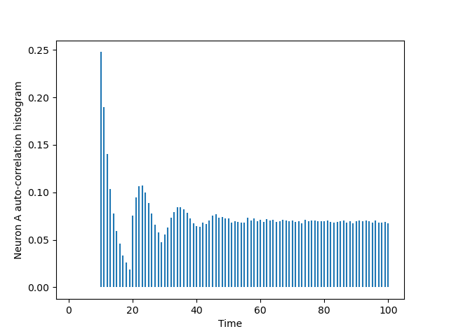
The auto-correlation histogram of this A_train is computed using the cch_discrete function we defined in the previous exercise; a version of which is available in file code/cch_discrete.py.
Using matplotlib we can make a plot of this histogram (the next code block assumes that your Python working directory, what is returned by os.getcwd, has code as a sub-directory):
import matplotlib.pylab as plt
from code.cch_discrete import cch_discrete
AA = cch_discrete(A_train,A_train,100)
tt = list(range(101))
plt.vlines(tt[1:],0,AA[1:])
plt.xlabel('Time')
plt.ylabel('Neuron A auto-correlation histogram')
Now take the above simulation code as a template, add to it the simulation of a B_train whose dynamics matches the one given in Sec. 2.2 with a linear \(\phi(\,)\) function between 0 and 1; that is, \(\phi(v) = 0\) for \(v < 0\), \(\phi(v) = v\) for \(0 \le v \le 1\) and \(\phi(v) = 1\) for \(v > 1\). Take a synaptic weight \(w_{A \to B} = 0.03\). Make figures corresponding to the cross-correlation histogram, \(\widehat{cc}_{A \to B}\) as well as to the two auto-correlation histograms like the Fig. 1 of Moore et al (1970).
Once you are done, go to the solution page.
2.4. Exploring a classic 2 (coding exercise)
Your task is now to replicate Fig. 3 of Moore et al (1970). Again two neurons are considered, A is presynaptic and excites B, but this time the auto-correlation histogram of A is flat (once the refractory period is over), meaning that \(\widehat{cc}_{A \to A}(0) = 0\) and \(\widehat{cc}_{A \to A}(t) = \text{Cst}\) for \(t\) large enough. An easy way to generate a spike train fulfilling these requirements is to modify the above function p_A(delta_t) by suppressing the transient probability increase between 10 and 20. You should be able to design the right dynamics for B, by summing a \(g_{B \to B}(\,)\) function with an appropriate \(g_{A \to B}(\,)\) one.
Once you are done, go to the solution page.
2.5. Exploring a classic 3 (coding exercise)
Now for something completely different: Fig. 4 of Moore et al (1970)! Two neurons A and B again, but with an intermediate layer of 3 neurons I\(_1\), I\(_2\) and I\(_3\). The pacemaker neuron A produces an excitation of each of the intermediate neurons with a 10 ms delay such that each neuron has a probability of 0.5 to fire a spike after an input from A. Then I\(_1\), I\(_2\) and I\(_3\) excite B with delays of 10, 20 and 30 ms. The network is schematized as follows:
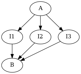 Take time steps corresponding to 1 ms. Modify function
 p_A( ) of Ex. 1 considering that the latter used a 10 ms time step while you now want a 1 ms one. Next, define a p_I( ) common to the three "interneurons" such that:
- they exhibit a 5 ms refractory period,
- 10 ms after a spike from A they have an elevated and constant spiking probability for 10 ms such that the probability of having a spike during this 10 ms period is 0.5,
- otherwise the spike probability is 5x10\(^{-4}\)
2.6. Making the figures
The graph made of 3 neurons
Graphviz was used. We first wrote into a file simple_graph_3_neurons.dot the following content:
digraph {
N1 -> N2;
N1 -> N3;
N2 -> N1;
N2 -> N3;
N3 -> N1;
}
Then we called Graphviz dot program as follows (from the command line):
dot -Tpng graph_3_neurons.dot
Membrane potential paths in the case without leakage
We first simulate a network made of 100 neurons, saving the result in a file named Vproc as described in the book:
import random  # random number module
random.seed(20200622)  # set RNG seed
N = 100  # Number of neurons in network
connection_prob = 0.2  # connection probability
graph = [[i for i in range(N) if random.random() <= connection_prob and
          i != j]
         for j in range(N)]  # generate Erdos-Renyi graph

thresh = 2*N*connection_prob # voltage threshold
# If V_t(i) >= thresh the spiking probability is going to be 1
# This is what is implemented by the following function
def phi(v):
    return min(v/thresh,1.0)

V = [random.randint(0,thresh) for i in range(N)]  # initialize V

fout = open('Vproc','w') # write simulation to file name 'Vproc'
fout.write(str([0]+V).strip('[]')+'\n')

n_step = 1000 # the number of time steps
for t in range(1,n_step+1): # Do the simulation
    P = [phi(v) for v in V]  # spiking probability
    # Find out next if each neuron spikes or not
    S = [random.random() <= P[i] for i in range(N)]
    for i in range(N):
        if S[i]:  # neuron n spiked
           V[i] = 0  # reset membrane potential
        else:  # neuron n did not spike
            for k in graph[i]: # look at presynaptic neurons
                if S[k]: # if presynaptic spiked
                   V[i] += 1 # identical weight of 1 for each synapse
    fout.write(str([t]+V).strip('[]')+'\n') # write new V

fout.close()
The TikZ version of the figure is then obtained with:
idx = []
V_ntw = [[] for i in range(N)]
for line in open('Vproc','r'):
    elt = line.split(',')
    idx.append(int(elt[0]))
    for i in range(N):
        V_ntw[i].append(int(elt[i+1]))

import matplotlib.pylab as plt
from matplotlib.patches import Polygon
from matplotlib.collections import PatchCollection
fig, ax = plt.subplots()
fig.subplots_adjust(wspace=0,hspace=0,left=0,right=1,top=1,bottom=0)
start = 40
delta = 20
ax.margins=0
offset = 0
patches = []
I = idx[-start:]
V = [offset+V_ntw[1][t] for t in range(1001)]
for t in I:
    if V[t] == offset and V[t-1]>offset:
        polygon = Polygon([[t,offset],
                           [t,offset+delta],
                           [t+1,offset+delta],
                           [t+1,offset]])
        patches.append(polygon)

ax.step(I,V[-start:],where='post',color='red')
offset += delta

for i in graph[1]:
    V = [offset+V_ntw[i][t] for t in range(1001)]
    for t in I:
        if V[t] == offset and V[t-1]>offset:
            polygon = Polygon([[t,offset],
                               [t,offset+delta],
                               [t+1,offset+delta],
                               [t+1,offset]])
            patches.append(polygon)
    ax.step(I,V[-start:],where='post',color='black' if (offset/delta) % 2 == 0 else 'grey')
    offset += delta

p = PatchCollection(patches, alpha=0.5,facecolor='lightgrey')
ax.add_collection(p)
ax.axis('off')
import tikzplotlib
tikzplotlib.save('simple-discrete-time-model.tex')
3. Appendix A Material
3.1. The inter mepp data of Fatt and Katz (1952)
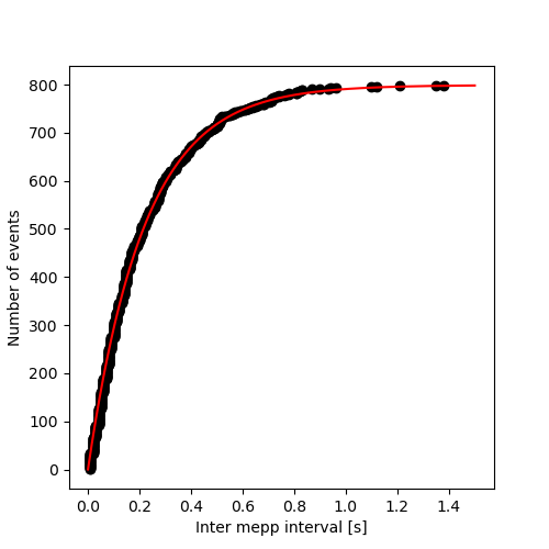
This project/set of exercises invites you to explore a dataset from the first paper describing the stochastic behavior of a synapse: Paul Fatt and Bernhard Katz (1952) Spontaneous subthreshold activity at motor nerve endings. In this article, Fatt and Katz report the observation of small spontaneous potentials from the end-plate region of the frog neuromuscular junction that they referred to as miniature end-plate potentials (mepp). They argued that these potentials originate from the spontaneous release of transmitter from the nerve terminal. They then studied the response of the same muscle fiber to presynaptic nerve stimulation in a low extracellular calcium condition–lowering thereby transmitter release–and saw that these reduced evoked responses fluctuate in steps whose amplitudes matched the ones of spontaneous potentials. In the same paper, Fatt and Katz study the distribution of the intervals between successive mepp and show it to be compatible with an exponential distribution (Fig. 12).
This was a first indication that these miniature events follow a homogeneous Poisson process. These inter mepp interval data were originally published by Cox and Lewis (1966) The statistical analysis of series of events, where they are wrongly described as inter spike interval data; they are also used–with the same wrong description–in the two excellent books of Larry Wasserman, All of Statistics and All of Nonparametric Statistics.
3.2. Exercise 1: Getting the data
Larry Wasserman took the data of Fatt and KAtz from the Appendix of Cox and Lewis (1966) and put them on a page of his web site dedicated to the datasets used in his books. You can therefore download the data from http://www.stat.cmu.edu/~larry/all-of-nonpar/=data/nerve.dat, they are organized in columns (6 columns) and all the rows are complete except the last one that contains data only on the first column. The data are inter mepp intervals in seconds and should be read across columns; that is first row, then second row, etc.
Your first task is to read these data in your Python environment and to keep them in a list.
3.3. Exercise 2: Basic statistics
On p. 123, Fatt and Katz state that they have 800 mepp and that the mean interval is 0.221 s. Compare with what you get. Do a bit more by constructing the five-numer summary–namely the minimum, first quartile, median, third quartile and maximum statistics–.
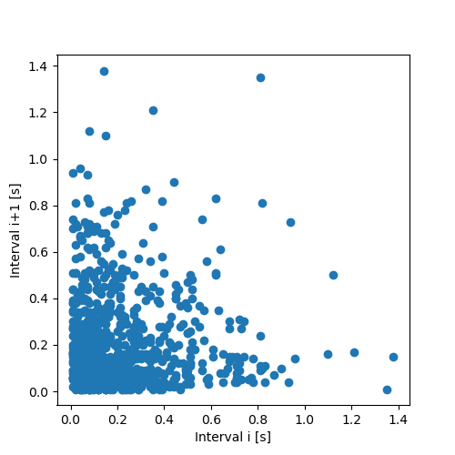
3.4. Exercise 3: Interval correlations
Look for correlations between successive intervals:
- Plot interval
i+1vs intervali. - Plot the rank of interval
i+1vs the rank of intervali\citep{Rhoades_1996}; comment on the difference between the first display and the present one. - Using the ranks you just computed, get the Spearman's rank correlation for the intervals for lags between 1 and 5, compare the obtained values with the standard error under the null hypothesis; since the data were truncated they contain many duplicates, making the theoretical confidence intervals not very reliable (see the previous link), you will therefore resample 1000 times from your ranks (use the
samplefunction from the random module of the standard library and do not forget to set your random number generator seed with functionseedof this module), compute the maximum (in absolute value) of the five coefficients (for the five different lags) and see were the actual max of five seats in this simulated sampling distribution; conclude.
3.5. Exercise 4: Counting Process Class
You will first create a Class whose main private data will be an iterable (e.g. a list) containing arrival times. In the context of Fatt and Katz data, the arrival times are obtained from the cumulative sum of the intervals. Ideally class instanciation should check that the parameter value provided by the user is a suitable iterable. Your class should have two methods:
- sample_path
- that returns the counting process sample path corresponding to the arrival times passed as argument for any given time (using the
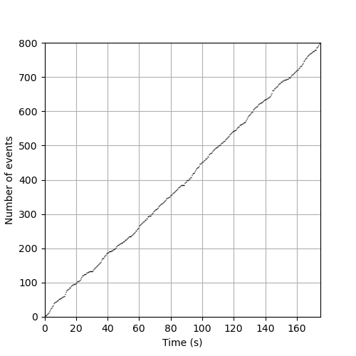
bisectfunction of the bisect module can save you some work). - plot
- that generates a proper step function's graph, that is, one without vertical lines.
3.6. Exercise 5: Graphical test of arrival times 'uniformity'
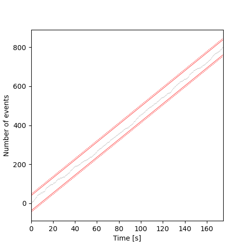
A classical result states that the arrival times of a stationary Poisson counting process observed between 0 and \(T\), conditioned on the number of events observed are uniformly distributed on \([0,T]\) \citep{CoxLewis_1966}. It is therefore possible, using the improperly called one sample Kolmogorov-Smirnov test ('Kolmogorov' test is the proper name for it) and the Kolmogorov distribution for the test statistics to build a confidence band around the ideal counting process sample path that is known once the observation time \(T\) and the number of observed events \(n\) are known: it should be a stright line going through the origin and through the point \((T,n)\). Strangly enough tables giving the asymptotic critical values of the Kolmogorov's statistics \(D_n\) (\(n\) is the sample size) are rare, Bock and Krisher Data Analysis BriefBook give the following critical values for \(\sqrt{n} D_n\) (\(n>80\)):
| Confidence level | \(\sqrt{n} D_n\) |
|---|---|
| 0.1 | 1.22 |
| 0.05 | 1.36 |
| 0.01 | 1.63 |
You can therefore make a quick graphical test by plotting the sample path together with the limits of the 95% and 99% confidence bands.
3.7. Exercise 6: Kolmogorov's test via C code interfacing (optional)
If you like the 'fancy stuff', you can decide to use 'exact' values (to 15 places after the decimal point, that is to the precision of a double on a modern computer) of the Kolmogorov's statistics distribution. Marsaglia, Tsang and Wang (2003) Evaluating Kolmogorov's Distribution give a C code doing this job that can be freely downloaded from the dedicated page of the Journal of Statistical Software. If you feel advanturous, you can download this code, compile it as a shared library and interface it using module ctypes to your Python session. Once this interface is running, you can compute the p-value of the observed value of the statistics. You can find a very basic ctypes tutorial from Jülich and a more advanced in the official documentation. To learn C properly check James Aspnes' Notes on Data Structures and Programming Techniques.
3.8. Exercise 7: Figure 12 reproduction and more
Reproduce Figure 12 of Fatt and Katz (1952). Then, remarking that the complementary of the (cumulative) distribution function of an exponential, \(F(t) = 1-e^{-t/\tau}\) is \(F^c(t) = 1-F(t) = e^{-t/\tau}\) make a graph of the empirical version of \(F^c\) using a log scale on the ordinate.
3.9. Solution 1: Getting the data
Command line based solution
A first solution to get the data, for people who like the command line, is to use wget:
wget http://www.stat.cmu.edu/~larry/all-of-nonpar/=data/nerve.dat \
     --no-check-certificate
--2024-01-11 17:35:52--  http://www.stat.cmu.edu/~larry/all-of-nonpar/=data/nerve.dat
Résolution de www.stat.cmu.edu (www.stat.cmu.edu)… 128.2.12.64
Connexion à www.stat.cmu.edu (www.stat.cmu.edu)|128.2.12.64|:80… connecté.
requête HTTP transmise, en attente de la réponse… 301 Moved Permanently
Emplacement : https://www.stat.cmu.edu/~larry/all-of-nonpar/=data/nerve.dat [suivant]
--2024-01-11 17:35:53--  https://www.stat.cmu.edu/~larry/all-of-nonpar/=data/nerve.dat
Connexion à www.stat.cmu.edu (www.stat.cmu.edu)|128.2.12.64|:443… connecté.
AVERTISSEMENT : impossible de vérifier l’attribut www.stat.cmu.edu du certificat, émis par ‘CN=InCommon RSA Server CA,OU=InCommon,O=Internet2,L=Ann Arbor,ST=MI,C=US’ :
  Impossible de vérifier localement l’autorité de l’émetteur.
requête HTTP transmise, en attente de la réponse… 200 OK
Taille : 4134 (4,0K)
Enregistre : ‘nerve.dat’

     0K ....                                                  100% 76,8M=0s

2024-01-11 17:35:54 (76,8 MB/s) - ‘nerve.dat’ enregistré [4134/4134]
I can check the content of the first 5 rows of the file with the head program as follows:
head -n 5 nerve.dat
0.21	0.03	0.05	0.11	0.59	0.06
0.18	0.55	0.37	0.09	0.14	0.19
0.02	0.14	0.09	0.05	0.15	0.23
0.15	0.08	0.24	0.16	0.06	0.11
0.15	0.09	0.03	0.21	0.02	0.14
Using tail, I can check the content of the last five rows as follows:
tail -n 5 nerve.dat
0.05	0.49	0.10	0.19	0.44	0.02
0.72	0.09	0.04	0.02	0.02	0.06
0.22	0.53	0.18	0.10	0.10	0.03
0.08	0.15	0.05	0.13	0.02	0.10
0.51
We see that the data are on 6 columns and that all the rows seem to be complete (it can be a good idea to check that with a pager like less) except the last one that has an element only in the first column (whose index is 0 in Python). The columns are moreover separated by tabs. One way to load the data in Python is:
imepp = []
for line in open("nerve.dat"):
    elt = line.split('\t')
    if elt[1] != '': # the row is complete
        imepp += [float(x) for x in elt]
    else: # last row with a single element
        imepp += [float(elt[0])]

len(imepp)
799
Pure Python solution
Instead of using the command line, we can use the urllib.request module of the standard library as well as the ssl module so that it becomes possible to avoid certificate checking (I found the trick on stackoverflow: Python 3 urllib ignore SSL certificate verification):
import ssl
import urllib.request as url  #import the module
ctx = ssl.create_default_context()
ctx.check_hostname = False
ctx.verify_mode = ssl.CERT_NONE
fh = url.urlopen("http://www.stat.cmu.edu/~larry/all-of-nonpar/=data/nerve.dat", context=ctx)
content = fh.read().decode("utf8")
imepp = [float(x) for x in content.split()]
len(imepp)
799
Here the fh.read().decode("utf8") is used because fh behaves an a opened file in binary mode. content.split() splits the string at every white space, line break, etc. The penultimate line makes use of a list comprehension.
3.10. Solution 2: Basic statistics
The quick way to get the sample mean is to use function mean from the standard library module statistics.
import statistics
statistics.mean(imepp)
0.21857321652065081
A slightly crude way to get the five-number summary is:
[sorted(imepp)[i] for i in [round(k*(len(imepp)-1))
                            for k in [0,0.25,0.5,0.75,1]]]
[0.01, 0.07, 0.15, 0.3, 1.38]
This is 'crude' since we use a round function to get the index of the sorted data, namely, we get the first quartile by rounding 0.25x798 (=199.5) and we get 200 while, strictly speaking, we should take the sum of the sorted data at indices 199 and 200 and divide it by 2.
3.11. Solution 3: Interval correlations
To plot interval i+1 vs interval i, we can simply do (we need to load matplotlib):
import matplotlib.pylab as plt
plt.figure(figsize=(5, 5))
plt.plot(imepp[:-1],imepp[1:],"o")
plt.xlabel("Interval i [s]")
plt.ylabel("Interval i+1 [s]")
plt.savefig("figsPSNN/ExFattKatzQ3a.png")
"figsPSNN/ExFattKatzQ3a.png"
To plot the ranks we first need to obtain them, that is, we need to replace each interval value by its rank in the sorted interval values. An elementary way of doing this job can go as follows:
- We create tuples with the index and the value of each original interval and store all these tuples in a list (keeping the original order of course).
- We sort the list of tuples based on the interval value.
- We fill a rank vector by assigning the value of an increasing index (starting from 0 an increasing by 1) to the position specified by the first element of the sorted tuples.
We can first test the procedure with the example of the Wikipedia page: '3.4, 5.1, 2.6, 7.3' should lead to '2, 3, 1, 4' (with an index starting at 1)
test_data = [3.4, 5.1, 2.6, 7.3]
# Point 1
i_test_data = [(i,test_data[i]) for i in range(len(test_data))]
# Point 2
s_i_test_data = sorted(i_test_data, key=lambda item: item[1])
# Start point 3
idx = 1
test_rank = [0 for i in range(len(test_data))]  # intialization
for elt in s_i_test_data:
    test_rank[elt[0]] = idx
    idx += 1
# End point 3
test_rank
[2, 3, 1, 4]
Fine, we can now run it on our data (with an index starting at 0):
i_imepp = [(i,imepp[i]) for i in range(len(imepp))]    # Point 1
s_i_imepp = sorted(i_imepp, key=lambda item: item[1])  # Point 2
idx = 0                                                # Start point 3
rank = [0 for i in range(len(imepp))] # intialization
for elt in s_i_imepp:                                  # End point 3
    rank[elt[0]] = idx
    idx += 1
The plot gives:
plt.figure(figsize=(5, 5))
plt.plot(rank[:-1],rank[1:],'o')
plt.xlabel("Rank of interval i [s]")
plt.ylabel("Rank of interval i+1 [s]")
plt.savefig('figsPSNN/ExFattKatzQ3b.png')
'figsPSNN/ExFattKatzQ3b.png'
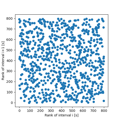
Since the interval distribution is skwed to the right (it rises fast and decays slowly, like most duration distributions), plotting intervals against each other make a bad use of the plotting surface and leads to too many points in the lower left corner; structures can't be seen anymore if some are there. Using the rank eliminates the 'distortion' due to the distribution and under the null hypothesis (no correlation), the graph should be filled essentially uniformly.
To compute the Spearman's rank correlations, we first prepare a version of the ranks from which we subtract the mean rank and that we divide by the rank standard deviation (we can't use the theoretical value for the latter since many intervals have the same value, due to truncation):
rank_sd = statistics.stdev(rank)
rank_mean = statistics.mean(rank)
rank_normed = [(r-rank_mean)/rank_sd for r in rank]
We define a function spearman that returns the Spearman's correlation coefficient for a given iterable containing normed data (mean 0 and SD 1) and a given lag:
def spearman(normed_data, lag=1):
    """Returns Spearman's auto-correlation coefficent at a given lag.

    Parameters
    ----------
    normed_data: an iterable with normed data (mean 0 and SD 1)
    lag: a positive integer, the lag

    Returns
    -------
    The Spearman's auto-correlation coefficent at lag (a float)
    """
    n = len(normed_data)-lag
    return sum([normed_data[i]*normed_data[i+lag] for i in range(n)])/n
We can then get the auto-correlation at the five different lags:
rank_cor = [spearman(rank_normed, lag=k) for k in [1,2,3,4,5]]
rank_cor
[-0.041293322480167906,
 0.0310350375233785,
 0.02987780737228069,
 -0.03737263560582801,
 0.049288720472378866]
We now go ahead with the 1000 replicates and we approximate the distribution of the max of the five auto-correlation coefficients (in absolute value) under the null hypothesis (no correlation):
import random
random.seed(20061001)  # set the seed
n_rep=1000
actual_max_of_five = max([abs(x) for x in rank_cor])  # observed value
# create a list that will store the statistics under the null
rho_max_of_five = [0 for i in range(n_rep)]
for i in range(n_rep):
    # shuffle the ranks (i.e. make the null true)
    samp = random.sample(rank_normed,len(rank_normed))
    # compute the statistics on shuffled ranks
    rho_max = max([abs(x) for x in [spearman(samp, lag=k) for k in [1,2,3,4,5]]])
    rho_max_of_five[i] = rho_max # store the result

sum([1 for rho in rho_max_of_five if rho <= actual_max_of_five])/n_rep
0.408
That's the p-value and we can conclude that the intervals behave as non-correlated intervals.
3.12. Solution 4: Counting Process Class
Class skeleton
class CountingProcess:
     """A class dealing with counting process sample paths"""
     <<init_method-cp>>
     <<sample_path-method-cp>>
     <<plot-method-cp>>
__init__ method (<<init_method-cp>>)
Here the code is written in a more 'robust' way than the previous ones. Upon creation of the instanciation of a class, that's what the call to the __init__ method is doing, checks are performed on the value passed as a parameter. The collections.abc module is used since it contains the definition of the Iterable type allowing us to check against any of the actual iterable types (list, arrays, tuple, etc.) in a single code line. We also check that the elements of the iterable are increasing.
def __init__(self,times):
     from collections.abc import Iterable
     if not isinstance(times,Iterable): # Check that 'times' is iterable
          raise TypeError('times must be an iterable.')

     n = len(times)
     diff = [times[i+1]-times[i] for i in range(n-1)]
     all_positive = sum([x > 0 for x in diff]) == n-1
     if not all_positive:  # Check that 'times' elements are increasing
          raise ValueError('times must be increasing.')

     self.cp = times
     self.n = n
     self.min = times[0]
     self.max = times[n-1]
sample_path method (<<sample_path-method-cp>>)
The sample_path method is just a disguised call to function bisect of module bisect. The call here is to find the index of the leftmost time (element of the original times parameter passed to __init__) smaller of equal to the value passed as sample_path parameter.
def sample_path(self,t):
     """Returns the number of observations up to time t"""
     from bisect import bisect
     return bisect(self.cp,t)
plot method (<<plot-method-cp>>)
The plot method generates a proper graphical representation of a step function, that is one without vertical lines.
def plot(self, domain = None, color='black', lw=1, fast=False):
    """Plots the sample path

    Parameters:
    -----------
    domain: the x axis domain to show
    color: the color to use
    lw: the line width
    fast: if true the inexact but fast 'step' method is used

    Results:
    --------
    Nothing is returned the method is used for its side effect
    """
    import matplotlib.pylab as plt
    import math
    n = self.n
    cp = self.cp
    val = range(1,n+1)
    if domain is None:
        domain = [math.floor(cp[0]),math.ceil(cp[n-1])]
    if fast:
        plt.step(cp,val,where='post',color=color,lw=lw)
        plt.vlines(cp[0],0,val[0],colors=color,lw=lw)
    else:
        plt.hlines(val[:-1],cp[:-1],cp[1:],color=color,lw=lw)
    plt.xlim(domain)
    if (domain[0] < cp[0]):
        plt.hlines(0,domain[0],cp[0],colors=color,lw=lw)
    if (domain[1] > cp[n-1]):
        plt.hlines(val[n-1],cp[n-1],domain[1],colors=color,lw=lw)
Checks
Let us see how that works; to that end we must first create a time sequence out of the interval sequence:
n = len(imepp)
cp = [0 for i in range(n)]
cp[0] = imepp[0]
for i in range(1,n): cp[i] = imepp[i]+cp[i-1]

cp1 = CountingProcess(cp)
print("The number of events is: {0}.\n"
      "The fist event occurs at: {1}.\n"
      "The last event occurs at: {2}.\n".format(cp1.n,
                                                cp1.min,
                                                round(cp1.max,2)))
The number of events is: 799.
The fist event occurs at: 0.21.
The last event occurs at: 174.64.
Lets us check that the parameter value passed upon initialization works properly. First with a non-iterable:
cp_test = CountingProcess(10)
Traceback (most recent call last):
  File "<stdin>", line 1, in <module>
  File "<stdin>", line 12, in __init__
ValueError: times must be an iterable.
Next with an iterable that is not increasing:
cp_test = CountingProcess([1,2,4,3])
Traceback (most recent call last):
  File "<stdin>", line 1, in <module>
  File "<stdin>", line 12, in __init__
ValueError: times must be increasing.
Then with an increasing iterable that is not a list but an array:
import array
cp_test = CountingProcess(array.array('d',[1,2,3,4,5]))
print("The number of events is: {0}.\n"
      "The fist event occurs at: {1}.\n"
      "The last event occurs at: {2}.\n".format(cp_test.n,
                                                cp_test.min,
                                                cp_test.max))
The number of events is: 5.
The fist event occurs at: 1.0.
The last event occurs at: 5.0.
We can call the sample_path method as follows:
cp1.sample_path(100.5)
453
So 453 events were observed between \(0\) and \(100.5\).
The plot method leads to, guess what, a plot (assuming the import matplotlib.pylab as plt as already been issued):
plt.figure(figsize=(5, 5))
cp1.plot()
plt.xlabel('Time (s)')
plt.ylabel('Number of events')
plt.ylim(0,800)
plt.grid()
plt.savefig('figsPSNN/ExFattKatzQ4.png')
'figsPSNN/ExFattKatzQ4.png'
3.13. Solution 5: Graphical test of arrival times 'uniformity'
We proceed as follows using the critical values considering one important subtelty: on the sample path representation, the maximum value reached on the right of the graph is not 1 as it is for a proper (cumulative) distribution function but \(n\), the number of events; in other words the \(y\) axis is scales by a factor \(n\) compared to the 'normal' Kolmogorov's test setting, that is why we multiply by \(\sqrt{n}\) instead of dividing by it in the following code.
import math  # to get access to sqrt
plt.figure(figsize=(5, 5))
cp1.plot(lw=0.2)
delta95 = 1.36*math.sqrt(cp1.n)
delta99 = 1.63*math.sqrt(cp1.n)
plt.plot([cp1.min,cp1.max],
         [1+delta95,cp1.n+delta95],
         lw=0.5,ls='-', color='red') # upper 95% limit in red and continuous
plt.plot([cp1.min,cp1.max],
         [1-delta95,cp1.n-delta95],
         lw=0.5,ls='-', color='red')
plt.plot([cp1.min,cp1.max],
         [1+delta99,cp1.n+delta99],
         lw=0.5,ls='--', color='red') # upper 99% limit in red and dashed
plt.plot([cp1.min,cp1.max],
         [1-delta99,cp1.n-delta99],
         lw=0.5,ls='--', color='red')
plt.xlabel("Time [s]")
plt.ylabel("Number of events")
plt.savefig('figsPSNN/ExFattKatzQ5.png')
'figsPSNN/ExFattKatzQ5.png'
3.14. Solution 6: Kolmogorov's test via C code interfacing
We start by downloading the code and unzipping it in a subdirectory named code:
cd code && wget https://www.jstatsoft.org/index.php/jss/article/downloadSuppFile/v008i18/k.c.zip
unzip k.c.zip
--2024-01-12 10:27:11--  https://www.jstatsoft.org/index.php/jss/article/downloadSuppFile/v008i18/k.c.zip
Résolution de www.jstatsoft.org (www.jstatsoft.org)… 138.232.16.156
Connexion à www.jstatsoft.org (www.jstatsoft.org)|138.232.16.156|:443… connecté.
requête HTTP transmise, en attente de la réponse… 301 Moved Permanently
Emplacement : https://www.jstatsoft.org/htaccess.php?volume=008&type=i&issue=18&filename=k.c.zip [suivant]
--2024-01-12 10:27:11--  https://www.jstatsoft.org/htaccess.php?volume=008&type=i&issue=18&filename=k.c.zip
Réutilisation de la connexion existante à www.jstatsoft.org:443.
requête HTTP transmise, en attente de la réponse… 302 Found
Emplacement : https://www.jstatsoft.org/article/view/v008i18/3121 [suivant]
--2024-01-12 10:27:11--  https://www.jstatsoft.org/article/view/v008i18/3121
Réutilisation de la connexion existante à www.jstatsoft.org:443.
requête HTTP transmise, en attente de la réponse… 302 Found
Emplacement : https://www.jstatsoft.org/index.php/jss/article/download/v008i18/3121 [suivant]
--2024-01-12 10:27:11--  https://www.jstatsoft.org/index.php/jss/article/download/v008i18/3121
Réutilisation de la connexion existante à www.jstatsoft.org:443.
requête HTTP transmise, en attente de la réponse… 303 See Other
Emplacement : https://www.jstatsoft.org/article/download/v008i18/3121 [suivant]
--2024-01-12 10:27:11--  https://www.jstatsoft.org/article/download/v008i18/3121
Réutilisation de la connexion existante à www.jstatsoft.org:443.
requête HTTP transmise, en attente de la réponse… 200 OK
Taille : 1312 (1,3K) [sp]
Enregistre : ‘k.c.zip’

     0K .                                                     100% 1011M=0s

2024-01-12 10:27:11 (1011 MB/s) - ‘k.c.zip’ enregistré [1312/1312]

Archive:  k.c.zip
  inflating: k.c
We then compile the code as a share library:
cd code && gcc -shared -O2 -o k.so -fPIC k.c
In our Python session (assumed to be running 'above' directory code) we import ctypes and 'load' the shared library:
import ctypes as ct
_klib = ct.cdll.LoadLibrary("./code/k.so")
We now have to look at the signature of the function we want to call (you have to open the C source file k.c for that and you will see: double K(int n,double d). If you read the documentation and you should always do that you see that n is the sample size and d the Kolmogorov's statistics. But what concerns us now is the type of the parameters and of the return value. If the equivalent Python types are not specified, Python assumes essentally that everything is an integer and that's not the case for d and for the returned value that are both of type double. We therefore do:
_klib.K.argtypes=[ct.c_int,ct.c_double]  # Parameter types
_klib.K.restype = ct.c_double            # Returned value type
Now we check that it works as it should by gettind the probability for the Kolmogorov's statistics to be smaller or equal to 0.274 when the sample size is 10 ( Marsaglia, Tsang and Wang (2003) Evaluating Kolmogorov's Distribution, p. 2 ):
_klib.K(10,0.274)
0.6284796154565043
We can now go ahead and get the Kolmogorov's statistics for our sample. If you look at the graph of a counting process sampe path, you will see that the maximal difference with the straight line going from the origin to the last observed event necessarily occurs at the arrival times (draw it if necessary to convince yourself that such is the case). So lets us get this maximal difference:
Dplus = [abs(cp1.n/cp1.max*cp1.cp[i] - cp1.sample_path(cp[i]))
     for i in range(cp1.n)] # 'upper' abs difference at each arrival time
Dminus = [abs(cp1.n/cp1.max*cp1.cp[i] - cp1.sample_path(cp[i-1]))
     for i in range(1,cp1.n)] # 'lower' abs difference at each arrival time

K_stat = max(Dplus+Dminus)/cp1.n
K_stat
0.025477047867323424
And the p-value is:
_klib.K(cp1.n,K_stat)
0.33228272454713365
We can therefore safely keep the null hypothesis: the data behave as if generated from a stationary Poisson process.
3.15. Solution 7: Figure 12 reproduction and more
Reproduce figure 12 is straightforward:
X = sorted(imepp)
Y = [i for i in range(1,len(imepp)+1)]
tau_hat = (cp1.max-cp1.min)/cp1.n
xx = [i*1.5/500 for i in range(501)]
yy = [(1-math.exp(-xx[i]/tau_hat))*cp1.n for i in range(len(xx))]
plt.figure(figsize=(5, 5))
plt.plot(X,Y,'o',color='black')
plt.plot(xx,yy,color='red')
plt.xlabel("Inter mepp interval [s]")
plt.ylabel("Number of events")
plt.savefig('figsPSNN/ExFattKatzQ7a.png')
'figsPSNN/ExFattKatzQ7a.png'
The graph of the complementary function with a log scale on the ordinate is obtained with:
Y_C = [((cp1.n+1)-i)/cp1.n for i in range(1,len(imepp)+1)]
plt.figure(figsize=(5, 5))
plt.plot(X,Y_C,'o',color='black')
plt.xlabel("Inter mepp interval [s]")
plt.ylabel("Complementary distribution function")
plt.yscale('log')
plt.savefig('figsPSNN/ExFattKatzQ7b.png')
'figsPSNN/ExFattKatzQ7b.png'
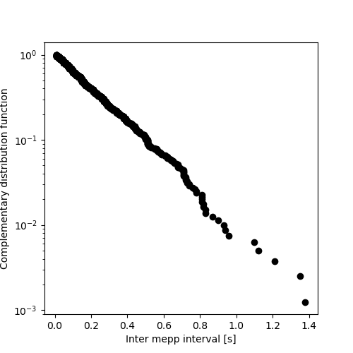
It is a straight line as it should be for data from an exponential distribution.