Exploring a classic 2: Coding Exercise
Table of Contents
1. The question recap
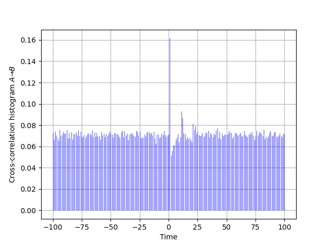
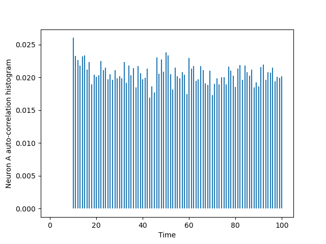
Your task is now to replicate Fig. 3 of Moore et al (1970). Again two neurons are considered, A is presynaptic and excites B, but this time the auto-correlation histogram of A is flat (once the refractory period is over), meaning that \(\widehat{cc}_{A \to A}(0) = 0\) and \(\widehat{cc}_{A \to A}(t) = \text{Cst}\) for \(t\) large enough. An easy way to generate a spike train fulfilling these requirements is to modify the above function p_A(delta_t) by suppressing the transient probability increase between 10 and 20. You should be able to design the right dynamics for B, by summing a \(g_{B \to B}(\,)\) function with an appropriate \(g_{A \to B}(\,)\) one.
2. The solution (Python)
We adapt the code of the previous exercise by defining first a function that returns the spiking probability of neuron A as a function of \(\delta{}t = t - L_t(A)\):
def p_A(delta_t):
    """Spiking probability of neuron A for a time since the last spike of 'delta_t'

    Parameters
    ----------
    delta_t: time since the last spike of neuron A

    Returns
    -------
    The spiking probability, a float between 0 and 1.
    """
    if delta_t < 10:
        return 0.0
    if delta_t >= 10:
        return 0.025
Function p_B computes the spiking probability of neuron B. It is a modification of function p_A of the last exercise, adding to it a synaptic effect that increses the spiking probability by 0.25:
def p_B(t_now, L_B, L_A):
    """Spiking probability of neuron B at 't_now' when the last spike from B was
    at time 'L_B' and the last spike from A was at time L_A

    Parameters
    ----------
    t_now: present time
    L_B: the time of the last spike from B
    L_A: the time of the last spike from A

    Returns
    -------
    The spiking probability, a float between 0 and 1.
    """
    delta_t = t_now - L_B
    if delta_t < 10:
        return 0.0 # refractory period
    if delta_t <= 20:
        p =  0.25
    if delta_t > 20:
        p =  0.025
    if L_A > L_B and t_now-L_A == 1:
        # A spikes at the last time step and out of B refractory period
        p += 0.25
    return p
We can now simulate the coupled spike trains with:
from random import random, seed
seed(20110928)
A_train = [0]
B_train = [0]
t_now = 1
while A_train[-1] <= 600000:
    p_A_now = p_A(t_now-A_train[-1])
    p_B_now = p_B(t_now, B_train[-1], A_train[-1])
    if random() <= p_A_now: # A spikes
        A_train += [t_now]
    if random() <= p_B_now: # B spikes
        B_train += [t_now]
    t_now += 1
print("A generated "+ str(len(A_train)) + " spikes and B generated " + str(len(B_train)) + " spikes")
A generated 12281 spikes and B generated 42760 spikes
The auto-correlation histogram of A is obtained with:
import matplotlib.pylab as plt
from code.cch_discrete import cch_discrete
AA = cch_discrete(A_train,A_train,100)
tt = list(range(101))
plt.vlines(tt[1:],0,AA[1:])
plt.xlabel('Time')
plt.ylabel('Neuron A auto-correlation histogram')
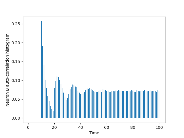
The one of B is obtined via a simple substitution:
BB = cch_discrete(B_train,B_train,100)
tt = list(range(101))
plt.vlines(tt[1:],0,BB[1:])
plt.xlabel('Time')
plt.ylabel('Neuron B auto-correlation histogram')
The cross-correlation histogram "matching" the one of Moore et al is obtained by two successive calls to cch_discrete since our function just deals with positive or null lags:
AB = cch_discrete(A_train,B_train,100)
BA = cch_discrete(B_train,A_train,100)
ttn = list(range(-100,1))
plt.vlines(ttn,0,[BA[100-i]*len(B_train)/len(A_train) for i in range(101)],
           color='blue',lw=0.5)
plt.vlines(tt,0,AB,color='blue',lw=0.5)
plt.xlabel('Time')
plt.ylabel(r'Cross-correlation histogram $A \to B$')
plt.grid()