Exploring a classic 1: Coding Exercise
Table of Contents
1. The question recap
We will now start a set of exercises based on an article by Moore, Segundo, Perkel and Levitan (1970) Statistical Signs of Synaptic Interaction in Neurons. We first do the simulation leading to Fig. 1 of the paper. Your task is to simulate two neurons, A and B to stick to the labels used by Moore et al, where A is presynaptic to B (a bit like our last test in the previous exercise). Neuron A discharge is stochastic periodic (in the sense that it tends to produce regular inter spike intervals). One way to produce such a discharge is to simulate a process whose spike probability at time \(t\) depends on the elapsed time since the last spike (the \(L_t\) of Eq. 2.1): \(\delta{}t \equiv t - L_t\). The "periodic" discharge is obtained by increasing significantly this probability during a short time window. We can for instance proceed as follows (following an approach initially proposed by D. Brillinger in Maximum likelihood analysis of spike trains of interacting nerve cells and discussed in Sec. B1 of the book):
# We define the spiking probability function
def p_A(delta_t):
    """Spiking probability for a time since the last spike of 'delta_t'

    Parameters
    ----------
    delta_t: time since the last spike

    Returns
    -------
    The spiking probability, a float between 0 and 1.
    """
    if delta_t < 10:
        return 0.0
    if delta_t <= 20:
        return 0.25
    if delta_t > 20:
        return 0.025

# We simulate a spike train
from random import random, seed
seed(20061001)
A_train = [0]
t_now = 1
while A_train[-1] <= 600000:
    if random() <= p_A(t_now-A_train[-1]):
        A_train += [t_now]
    t_now += 1
print(len(A_train))
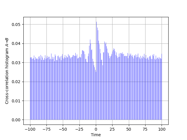
Now take the above simulation code as a template, add to it the simulation of a B_train whose dynamics matches the one given in Sec. 2.2 with a linear \(\phi(\,)\) function between 0 and 1; that is, \(\phi(v) = 0\) for \(v < 0\), \(\phi(v) = v\) for \(0 \le v \le 1\) and \(\phi(v) = 1\) for \(v > 1\). Take a synaptic weight \(w_{A \to B} = 0.03\). Make figures corresponding to the cross-correlation histogram, \(\widehat{cc}_{A \to B}\) as well as to the two auto-correlation histograms like the Fig. 1 of Moore et al (1970).
2. The solution (Python)
We modify the above simulation code as follows:
def p_A(delta_t):
    """Spiking probability for a time since the last spike of 'delta_t'

    Parameters
    ----------
    delta_t: time since the last spike

    Returns
    -------
    The spiking probability, a float between 0 and 1.
    """
    if delta_t < 10:
        return 0.0
    if delta_t <= 20:
        return 0.25
    if delta_t > 20:
        return 0.025

# We simulate a spike train
from random import random, seed
seed(20061001)
A_train = [0]
B_train = [0]
w_A2B = 0.03 # the synaptic weight from A to B
B_v = 0.0 # This tracks the 'membrane potential' of B
t_now = 1
while A_train[-1] <= 600000:
    p_B = min(1,B_v)
    if random() <= p_A(t_now-A_train[-1]): # A spikes
        A_train += [t_now]
        B_v += w_A2B # When A spikes the memb. pot. of B increases by w_A2B
    # NOTICE that p_B is not affected by what A just did
    if random() <= p_B: # B spikes
        B_train += [t_now]
        B_v = 0 # When B spikes its membrane potetnial is reset to 0
    t_now += 1
print("A generated "+ str(len(A_train)) + " spikes and B generated " + str(len(B_train)) + " spikes")
A generated 41150 spikes and B generated 19320 spikes
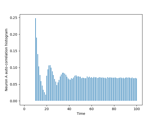
We have already built the auto-correlation histogram of A:
import matplotlib.pylab as plt
from code.cch_discrete import cch_discrete
AA = cch_discrete(A_train,A_train,100)
tt = list(range(101))
plt.vlines(tt[1:],0,AA[1:])
plt.xlabel('Time')
plt.ylabel('Neuron A auto-correlation histogram')
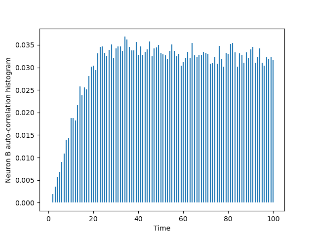
The one of B is obtined via a simple substitution:
BB = cch_discrete(B_train,B_train,100)
tt = list(range(101))
plt.vlines(tt[1:],0,BB[1:])
plt.xlabel('Time')
plt.ylabel('Neuron B auto-correlation histogram')
The cross-correlation histogram "matching" the one of Moore et al is obtained by two successive calls to cch_discrete since our function just deals with positive or null lags:
AB = cch_discrete(A_train,B_train,100)
BA = cch_discrete(B_train,A_train,100)
ttn = list(range(-100,1))
plt.vlines(ttn,0,[BA[100-i]*len(B_train)/len(A_train) for i in range(101)],
           color='blue',lw=0.5)
plt.vlines(tt,0,AB,color='blue',lw=0.5)
plt.xlabel('Time')
plt.ylabel(r'Cross-correlation histogram $A \to B$')
plt.grid()